Femur Shape Model Directly from Images
What is the Use Case?
The deep_ssm use case demonstrates how to get shape models from unsegmented images using deep learning on the femur data. This includes performing data augmentation as well as building, training and testing a DeepSSM model. For a detailed description of these processes, please see Data Augmentation for Deep Learning and SSMs Directly from Images. The image and shape data used for training and testing results from running the femur use case. Note running this use case does not require running the femur use case, the required data will automatically be downloaded.
On CUDA
This use case uses PyTorch and requires a GPU to run in a timely manner. The first time you run a DeepSSM use case, ShapeWorks downloads and installs PyTorch via light-the-torch, which detects your CUDA version and selects a matching GPU build (falling back to CPU if no compatible CUDA is found). See PyTorch GPU Support for ShapeWorks for how to verify GPU support and how to reinstall a different PyTorch version with swpip.
To do a quick check to see if PyTorch is running on your GPU, you can run the use case with the --tiny-test tag. This will quickly run the use case on a few examples and print an error if it is not running on the GPU.
Relevant Arguments
Use Case Pipeline
The use case pipeline includes creation of a training, validation, and testing sets. This involves particle optimization, image grooming, and data augmentation. Additionally, the use case demonstrates creating and training a DeepSSM network using ShapeWorks Python packages. For a full explanation of these packages see Using the Data Augmentation Python Package and Using the DeepSSM Python Package. Each step of the pipeline is outlined below.
Step 1: Getting the original data
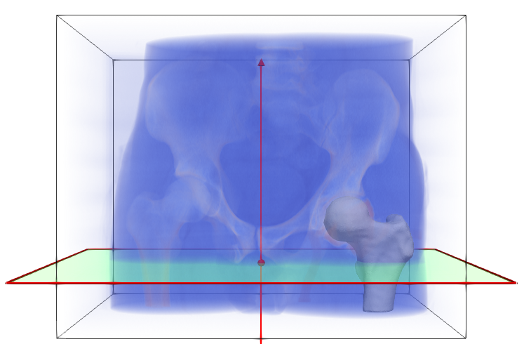
The femur data is downloaded from the ShapeWorks Data Portal. The data includes the original unsegmented .nrrd images, corresponding .ply mesh files, and .json constraint files with cutting planes. Below is one example of an MRI (blue), mesh (white), and corrresponding cutting plane (green).
Step 2: Define the data split
The data is randomly split into training (80%), validation (10%), and test (10%) sets. Of the 49 examples in the femur dataset, 39 are used to create training set, 5 are held out for the validation set, and the remaining 5 are held out for a test set. If running --tiny_test only 5 samples are downloaded and 3 are used in training, 1 for validation, and 1 for testing.
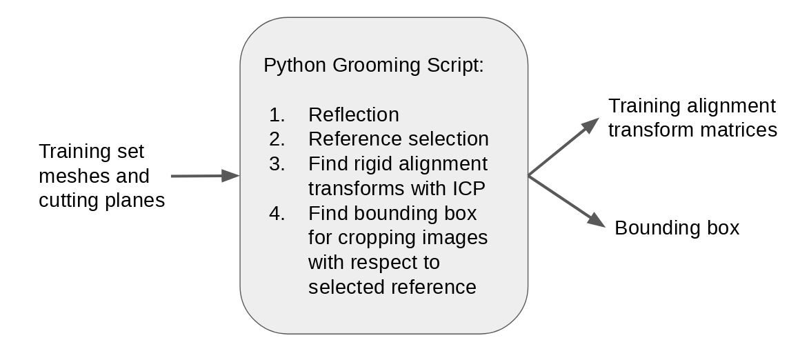
Step 3: Find training alignment transforms
Training DeepSSM requires labels or ground truth particles, thus we run optimization on the training set. As the femur meshes are unaligned, this requires finiding the alignment transforms to use in optimization. The steps for computing the transforms are the same as in the Femur Use Case. See Groom for more information on specific steps. In addition to computing the transforms, the smallest bounding box which contains all aligned meshes is computed.
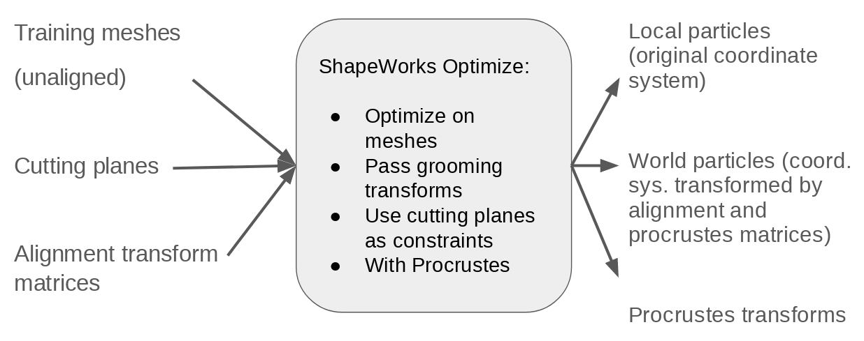
Step 4: Optimize training particles
Particles are optimized on the training femur meshes using corresponding alignment transforms and cutting planes as is done in the Femur Use Case.
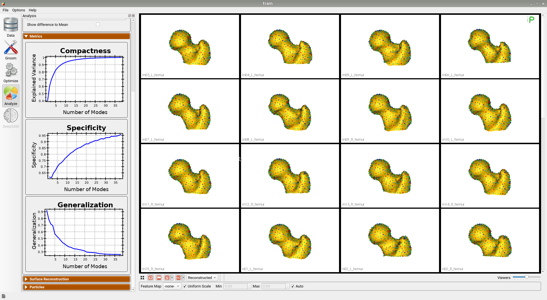
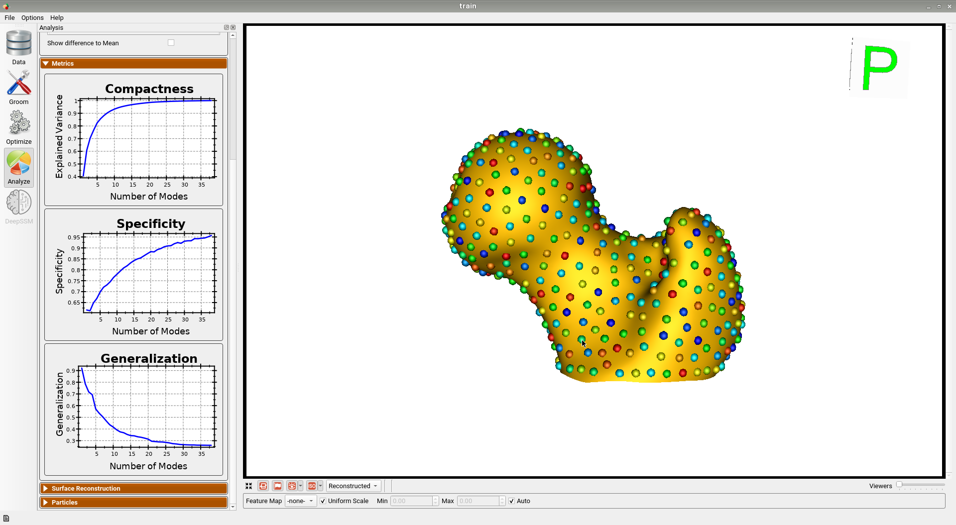
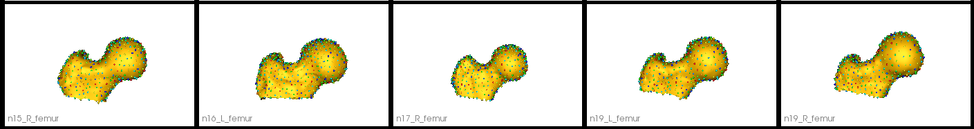
Below are some training set femur samples with their optimized correspondences.
Here is the mean shape of the optimized training shape model.
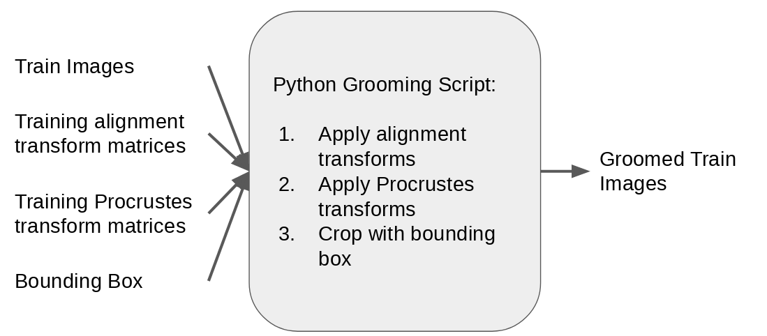
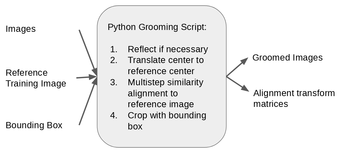
Step 5: Groom training images
Input images for the DeepSSM training set are created by taking the original training MRIs and applying the corresponding alignment transform (from step 3), applying the corresponding Procrustes transform (from optimization in step 4), and cropping using the boudning box (computed in step 3). This results in input images which consistently cropped and in alignment with the ground truth world particles.
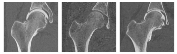
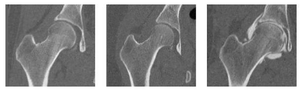
Here are some examples of slices of the groomed training images. These are now in alignment with the optimized world particles from Step 4.
Step 6: Data augmentation
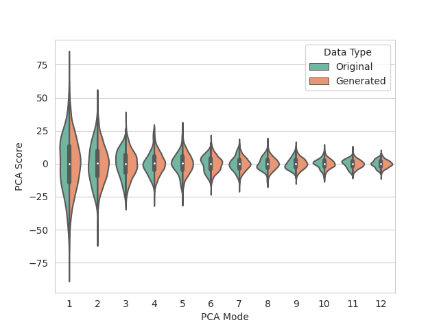
Data augmentation is run using the images and particle files allocated for training. 2967 augmented samples are created so that DeepSSM can be trained on 3000 total examples. The data is embedded to 12 dimensions using PCA, preserving 95% of the population variation. A Gaussian distribution is then fit to the embedded data and used in sampling new shape samples for data augmentation.
The functions relevant to this step are runDataAugmentation and visualizeAugmentation.
The distribution of real and augmented PCA scores are visualized as parallel violin plots.
Step 7: Find validation and test alignment transforms and groom images
To prepare the input images for the validation and test sets, the original MRIs are reflected if neccesary then aligned to a reference image using image registration. The reference image is selected as the groomed image corresponded to the training sample used in mesh alignment in step 3. The images are then cropped using the same bounding box computed in step 3 and the combined transforms are saved. Note this step does not use the validation or test meshes and can be performed without segmentation.
Here are some examples of the groomed validation and test images.
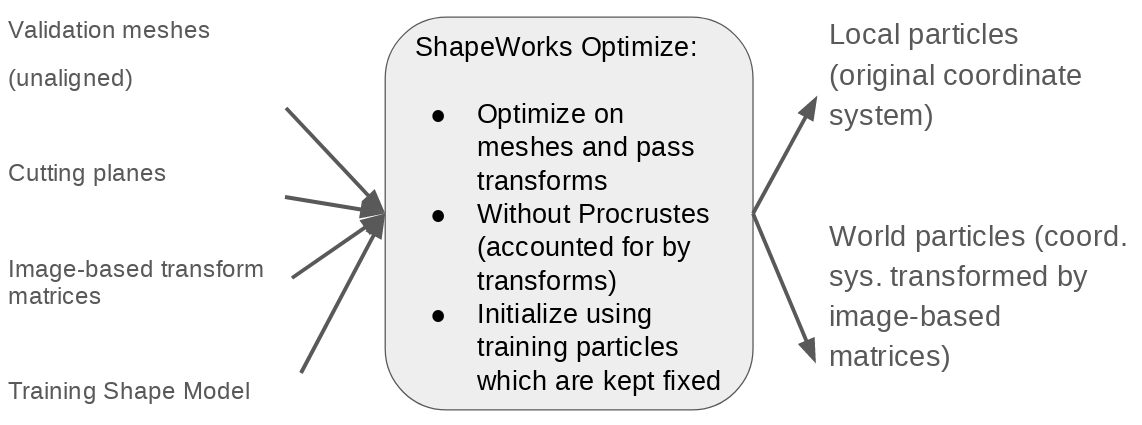
Step 8: Optimize validation particles with fixed domains
In order to quantify the accuracy of DeepSSM, ground truth particles are optimized on the validation set. This is done by adding the validation meshes to the training model while keeping the training particles fixed as is done in the Fixed Domain Use Case. The transforms found in step 7 are passed and Procrustes is turned off as these transform matrices account for scale.
Below are the resulting particles on the validation femurs.
Step 9: Create PyTorch loaders from data
The groomed images and particle files are reformatted into tensors for training and testing the DeepSSM network. In the case of the test loader, a place holder is used for the particles as we do not have ground truth particles. The functions relevant to this step are getTrainValLoaders and getTestLoader.
Note
If a CUDA memory error occurs when running the use case, the batch size value may need to be decreased.
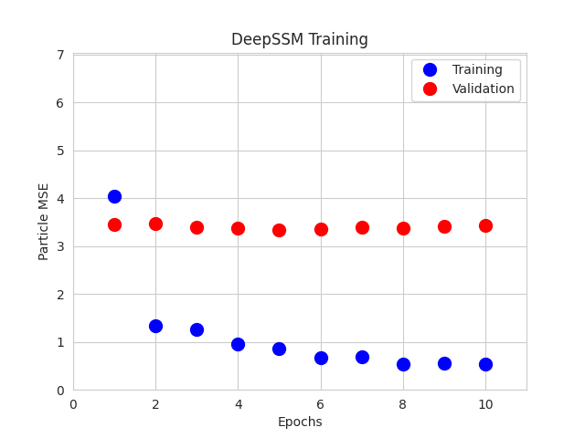
Step 10: Training DeepSSM
A DeepSSM model is created and trained for 10 epochs. A learning rate of 0.001 is used, and the validation error is calculated and reported every epoch.
The function relevant to this step is trainDeepSSM.
The training and validation errors are plotted after each epoch.
Step 11: Predict validation particles and analyze accuracy
The trained DeepSSM model is used to predict the world particles for the validation images. The function relevant to this step is testDeepSSM. The predicted local particles are aquired by applying the inverse transforms from step 7 to the world particles.
The accuracy is then analyzed via two means. The first is the mean square error between the predicted worl dparticles and ground truth world particles. The second is the surface-to-surface distance between the true mesh and the mesh generated from the predicted local particles. These results are printed to the console. The function relevant to this step is analyzeResults.
Step 12: Predict test particles and analyze accuracy
Similarly, the trained DeepSSM model is used to predict the world particles for the test images via testDeepSSM. As there are no ground truth particles, accuracy is just analyzed using the surface-to-surface distance between the true mesh and the mesh generated from the predicted local particles.
Below we can see the results on the 5 test shapes. The original image is with the predicted meshes which have a heat map displaying the surface-tosurface distance to the true mesh.
