Getting Started with Meshes¶

Before you start!¶

This notebook assumes that shapeworks conda environment has been activated using conda activate shapeworks on the terminal.
See Setting Up ShapeWorks Environment to learn how to set up your environment to start using shapeworks library. Please note, the prerequisite steps will use the same code to setup the environment for this notebook and import shapeworks library.
Note example output was generated on Linux/Mac environment and may look different on Windows.

In this notebook, you will learn:¶

How to define your dataset location and explore what is available in it
How to load a single mesh
How to convert shapeworks mesh to vtk mesh for visualization
How to visualize a surface mesh using pyvista

Importing `shapeworks` library¶

In [ ]:

import shapeworks as sw

1. Defining and exploring your dataset¶

Defining dataset location¶

You can download exemplar datasets from ShapeWorks data portal after you login. For new users, you can register an account for free. Please do not use an important password.

After you login, click Collections on the left panel and then use-case-data-v2. Select the dataset you would like to download by clicking on the checkbox on the left of the dataset name. See the video below.

This notebook assumes that you have downloaded ellipsoid_1mode and you have placed the unzipped folderellipsoid_1modein Examples/Python/Data. Feel free to use your own dataset.

In [ ]:

import os # for paths and mkdir

# dataset name is the folder name for your dataset
datasetName  = 'ellipsoid_1mode'

# path to the dataset where we can find shape data 
# here we assume shape data are given as surface meshes
shapeDir      = '../../Data/' + datasetName + '/meshes/'
    
print('Dataset Name:     ' + datasetName)
print('Shape Directory:  ' + shapeDir)

What is available in the dataset?¶

First let's see how many shapes we have in the dataset.

File formats: For surface meshes, all vtk-supported mesh formats can be used (e.g., vtk, ply, and stl).

In [ ]:

import glob # for paths and file-directory search
from pathlib import Path # for generating robust paths irrespective of the platform:Win/Linux/Mac
# file extension for the shape data
shapeExtention = '.vtk'

# let's get a list of files for available meshes in this dataset
# * here is a wild character used to retrieve all filenames 
# in the shape directory with the file extensnion
shapeFilenames = sorted(glob.glob(shapeDir + '*' + shapeExtention)) 

print ('Number of shapes: ' + str(len(shapeFilenames)))
print('Shape files found:')
for shapeFilename in shapeFilenames:
    shapeFilename = Path(shapeFilename)
    print(shapeFilename)

2. Loading a single mesh¶

We will select one mesh to explore for now. We will then use shapeworks Mesh class to load this surface mesh and print out its header information that includes .

In [ ]:

# select a shape by setting the shape index (in the filenames list)
shapeIdx       = 0

# the filename for the selected shape
shapeFilename  = shapeFilenames[shapeIdx]

# use shapeworks Mesh class to load it
print('Loading: ' + shapeFilename)
shapeMesh = sw.Mesh(shapeFilename)

# let's print out header information of this mesh - TODO: #828 
print('Header information: ')
print(shapeMesh)

3. Convert to a VTK mesh¶

To visualize a shapeworks mesh with pyvista, we need first to convert it to a vtk mesh.

In [ ]:

# convert shapeworks mesh to a vtk mesh
shapeMesh_vtk = sw.sw2vtkMesh(shapeMesh)

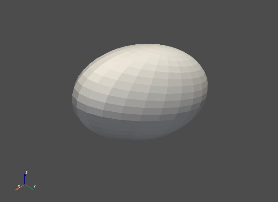
4. Visualizing surface mesh using `pyvista`¶

pyvista is a python library for 3D visualization and analysis. It is built on top of vtk and brings a paraview-like visualizations to notebooks. It also supports multiple rendering windows that can be linked. This feature is very useful when visualizing multiple samples from your dataset side-by-side and making them share the same camera view.

In [ ]:

# to have an interactive visualization, 
# click r to reset the view after zooming
# click w to show wireframe and s to return back to sur
notebook = False # True sets the figure inline in the notebook.
shapeMesh_vtk.plot(notebook = notebook)

5. Visualizing multiple meshes¶

When exploring datasets and results of different grooming (data preprocessing) steps, it is important to simultaneously visualize multiple shape samples. Here, we visualize two meshes side-by-side and link their views using pyvista. This linking is useful to make all rendering windows share the same camera view.

Loading the second mesh and convert it to `vtk` mesh¶

First, let's select another mesh and load it.

In [ ]:

# select a shape by setting the shape index (in the filenames list)
shapeIdx2       = 1

# the filename for the selected shape
shapeFilename2  = shapeFilenames[shapeIdx2]

# use shapeworks Mesh class to load it
print('Loading: ' + shapeFilename2)
shapeMesh2 = sw.Mesh(shapeFilename2)

# let's print out header information of this mesh 
print('Header information: ')
print(shapeMesh2)

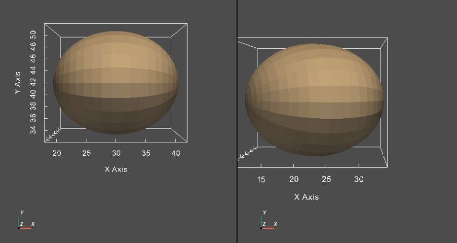
Now we can view the two meshes side by side using the ShapeWorks plot_meshes() function. To view the meshes in a side-by-side view, we set the use_same_window parameter to False. To view the meshes in the same window, we set the use_same_window parameter to True.

In [ ]:

meshList = [shapeMesh, shapeMesh2]
# View meshes side-by-side
sw.plot_meshes(meshList, use_same_window=False, notebook=notebook)

In [ ]:

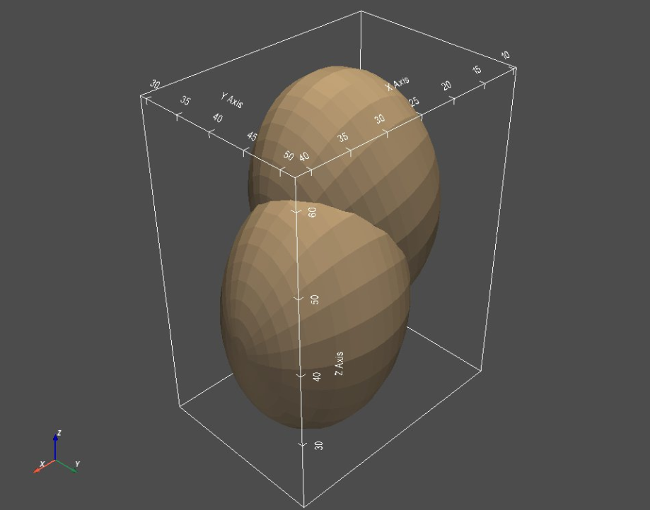
# View meshes in the same window
sw.plot_meshes(meshList, use_same_window=True, notebook=notebook)

Getting Started with Meshes¶

Before you start!¶

In this notebook, you will learn:¶

Importing shapeworks library¶

1. Defining and exploring your dataset¶

Defining dataset location¶

What is available in the dataset?¶

2. Loading a single mesh¶

3. Convert to a VTK mesh¶

4. Visualizing surface mesh using pyvista¶

5. Visualizing multiple meshes¶

Loading the second mesh and convert it to vtk mesh¶

Importing `shapeworks` library¶

4. Visualizing surface mesh using `pyvista`¶

Loading the second mesh and convert it to `vtk` mesh¶