Getting Started with Segmentations¶

Before you start!¶

• This notebook assumes that shapeworks conda environment has been activated using conda activate shapeworks on the terminal.
• See Getting Started with Notebooks for information on setting up your environment and notebook shortcuts.
• Note example output was generated on Linux/Mac environment and may look different on Windows.

In this notebook, you will learn:¶

1. How to define your dataset location and explore what is available in it
2. How to load a single segmentation
3. How to convert shapeworks image to vtk image for visualization
4. How to visualize a single segmentation and multiple segmentations using pyvista

In [ ]:

import shapeworks as sw

import shapeworks as sw

1. Defining and exploring your dataset¶

Defining dataset location¶

You can download exemplar datasets from ShapeWorks data portal after you login. For new users, you can register an account for free. Please do not use an important password.

After you login, click Collections on the left panel and then use-case-data-v2. Select the dataset you would like to download by clicking on the checkbox on the left of the dataset name. See the video below. After you download the dataset zip file, make sure you unzip/extract the contents in the appropriate location.

This notebook assumes that you have downloaded ellipsoid_1mode and you have placed the unzipped folder ellipsoid_1mode in Examples/Python/Data. Feel free to use your own dataset.

In [ ]:

import os 

# dataset name is the folder name for your dataset
datasetName  = 'ellipsoid_1mode'

# path to the dataset where we can find shape data 
# here we assume shape data are given as binary segmentations
shapeDir      = '../../Data/' + datasetName + '/segmentations/'

print('Dataset Name:     ' + datasetName)
print('Shape Directory:  ' + shapeDir)

import os # dataset name is the folder name for your dataset datasetName = 'ellipsoid_1mode' # path to the dataset where we can find shape data # here we assume shape data are given as binary segmentations shapeDir = '../../Data/' + datasetName + '/segmentations/' print('Dataset Name: ' + datasetName) print('Shape Directory: ' + shapeDir)

What is available in the dataset?¶

First let's see how many shapes we have in the dataset.

File formats: For binary segmentations, all itk-supported image formats can be used.

In [ ]:

import glob 
from pathlib import Path 


shapeExtention = '.nrrd'

# let's get a list of files for available segmentations in this dataset
# * here is a wild character used to retrieve all filenames 
# in the shape directory with the file extensnion

shapeFilenames = sorted(glob.glob(shapeDir + '*' + shapeExtention)) 

print ('Number of shapes: ' + str(len(shapeFilenames)))
print('Shape files found:')
for shapeFilename in shapeFilenames:
    shapeFilename = Path(shapeFilename)
    print(shapeFilename)

import glob from pathlib import Path shapeExtention = '.nrrd' # let's get a list of files for available segmentations in this dataset # * here is a wild character used to retrieve all filenames # in the shape directory with the file extensnion shapeFilenames = sorted(glob.glob(shapeDir + '*' + shapeExtention)) print ('Number of shapes: ' + str(len(shapeFilenames))) print('Shape files found:') for shapeFilename in shapeFilenames: shapeFilename = Path(shapeFilename) print(shapeFilename)

2. Loading a single segmentation¶

We will select one segmentation to explore for now. We will then use shapeworks Image class to load this segmentation and print out its header information that includes image dimensions (rows, columns and slices), physical origin, physical size, and voxel spacing (in physical units).

In [ ]:

# select a shape by setting the shape index (in the filenames list)
shapeIdx       = 1

# the filename for the selected shape
shapeFilename  = shapeFilenames[shapeIdx]

# since segmentation is just an image data, we will use shapeworks Image class to load it
print('Loading: ' + shapeFilename)
shapeSeg = sw.Image(shapeFilename)

# let's print out header information of this segmentation 
print('Header information: ')
print(shapeSeg)

# select a shape by setting the shape index (in the filenames list) shapeIdx = 1 # the filename for the selected shape shapeFilename = shapeFilenames[shapeIdx] # since segmentation is just an image data, we will use shapeworks Image class to load it print('Loading: ' + shapeFilename) shapeSeg = sw.Image(shapeFilename) # let's print out header information of this segmentation print('Header information: ') print(shapeSeg)

3. Converting shapeworks image to vtk image for visualization¶

We use python library pyvista for interactive 3D visualization. This library support, among others, vtk data structures for images and meshes. Hence, to visualize our shapeworks image, we need first to convert it to a vtk data structure.

This conversion can be performed by first extracting a numpy array from the shapeworks image, then constructing a vtk image from this array. pyvista's wrap function makes this easy.

In the ShapeWorks python module, we have the sw2vtkImage function for this conversion to vtk image.

In [ ]:

#from the shapeworks python module use the conversion function
shapeSeg_vtk = sw.sw2vtkImage(shapeSeg)

# print header info of both images, please note that the wrap function
# only wraps the numpy array, which is oblivous to image spacing and origin
print('shapeworks image header information: \n')
print(shapeSeg)

print('\nvtk image header information: \n')
print(shapeSeg_vtk)

#from the shapeworks python module use the conversion function shapeSeg_vtk = sw.sw2vtkImage(shapeSeg) # print header info of both images, please note that the wrap function # only wraps the numpy array, which is oblivous to image spacing and origin print('shapeworks image header information: \n') print(shapeSeg) print('\nvtk image header information: \n') print(shapeSeg_vtk)

4. Visualizing segmentation using pyvista¶

pyvista python library is built on top of vtk and brings a paraview-like visualizations to notebooks. It also supports multiple rendering windows that can be linked. This feature is very useful when visualizing multiple samples from your dataset side-by-side and making them share the same camera view.

In [ ]:

import pyvista as pv

notebook = False # True will bring the renderings inline
# click r to reset the view after zooming
shapeSeg_vtk.plot(volume     = True,     # volume render
                  shade      = True,
                  notebook = notebook)     # enable shading

import pyvista as pv notebook = False # True will bring the renderings inline # click r to reset the view after zooming shapeSeg_vtk.plot(volume = True, # volume render shade = True, notebook = notebook) # enable shading

5. Visualizing two segmentations side-by-side using pyvista¶

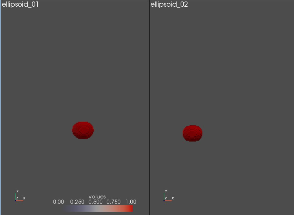
When exploring datasets and results of different grooming (data preprocessing) steps, it is important to simultaneously visualize multiple shape samples. Here, we will learn how to visualize two segmentations side-by-side and link their views using pyvista. This linking is useful to make all rendering windows share the same camera view.

Loading the second segmentation and convert it to vtk image¶

First, let's select another segmentation and load it.

In [ ]:

# select a shape by setting the shape index (in the filenames list)
shapeIdx2       = 2

# the filename for the selected shape
shapeFilename2  = shapeFilenames[shapeIdx2]

# since segmentation is just an image data, we will use shapeworks Image class to load it
print('Loading: ' + shapeFilename2)
shapeSeg2 = sw.Image(shapeFilename2)

# let's print out header information of this segmentation 
print('Header information: ')
print(shapeSeg2)

# select a shape by setting the shape index (in the filenames list) shapeIdx2 = 2 # the filename for the selected shape shapeFilename2 = shapeFilenames[shapeIdx2] # since segmentation is just an image data, we will use shapeworks Image class to load it print('Loading: ' + shapeFilename2) shapeSeg2 = sw.Image(shapeFilename2) # let's print out header information of this segmentation print('Header information: ') print(shapeSeg2)

Then, let's convert this shapeworks image to a vtk image for visualization.

In [ ]:

# sw to vtk
shapeSeg2_vtk = sw.sw2vtkImage(shapeSeg2)

# sw to vtk shapeSeg2_vtk = sw.sw2vtkImage(shapeSeg2)

Defining pyvista plotter¶

Next, we will define a pyvista plotter to render multiple windows, each with a single segmentation. The multiple rendering windows will be visualized as a grid of plots. Since, we have only two segmentations, the grid size will be one row and two columns.

The plotter also enable use to specify a color map.

In [ ]:

# define parameters that controls the plotter
notebook       = False  # True will bring the renderings inline in the notebook
show_borders   = True  # show borders for each rendering window
shade_volumes  = True  # use shading when performing volume rendering
color_map      = "coolwarm" # color map for volume rendering, e.g., 'bone', 'coolwarm', 'cool', 'viridis', 'magma'
show_axes      = True  # show a vtk axes widget for each rendering window
show_bounds    = False # show volume bounding box
show_all_edges = True  # add an unlabeled and unticked box at the boundaries of plot. 
font_size      = 10    # text font size for windows
link_views     = True  # link all rendering windows so that they share same camera and axes boundaries


#extract the shape name for display
segFilename = shapeFilenames[shapeIdx].split('/')[-1] 
shapeName   = segFilename[:-len(shapeExtention)]
segFilename2 = shapeFilenames[shapeIdx2].split('/')[-1] 
shapeName2   = segFilename2[:-len(shapeExtention)]
shapeSegList = [shapeSeg_vtk,shapeSeg2_vtk]
shapeNames = [shapeName,shapeName2]

# define parameters that controls the plotter notebook = False # True will bring the renderings inline in the notebook show_borders = True # show borders for each rendering window shade_volumes = True # use shading when performing volume rendering color_map = "coolwarm" # color map for volume rendering, e.g., 'bone', 'coolwarm', 'cool', 'viridis', 'magma' show_axes = True # show a vtk axes widget for each rendering window show_bounds = False # show volume bounding box show_all_edges = True # add an unlabeled and unticked box at the boundaries of plot. font_size = 10 # text font size for windows link_views = True # link all rendering windows so that they share same camera and axes boundaries #extract the shape name for display segFilename = shapeFilenames[shapeIdx].split('/')[-1] shapeName = segFilename[:-len(shapeExtention)] segFilename2 = shapeFilenames[shapeIdx2].split('/')[-1] shapeName2 = segFilename2[:-len(shapeExtention)] shapeSegList = [shapeSeg_vtk,shapeSeg2_vtk] shapeNames = [shapeName,shapeName2]

Let's use the plot_volumes function from Shapeworks python module for adding segmentations to the pyvista plotter

In [ ]:

sw.plot_volumes(shapeSegList,    
             volumeNames     = shapeNames, 
             notebook = notebook, 
             show_borders   = show_borders,  
             shade_volumes  = shade_volumes,  
             show_axes      = show_axes,  
             show_bounds    = show_bounds,
             show_all_edges = show_all_edges, 
             font_size      = font_size,   
             link_views     = True )

sw.plot_volumes(shapeSegList, volumeNames = shapeNames, notebook = notebook, show_borders = show_borders, shade_volumes = shade_volumes, show_axes = show_axes, show_bounds = show_bounds, show_all_edges = show_all_edges, font_size = font_size, link_views = True )

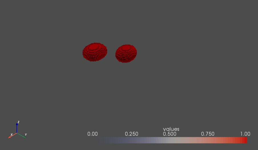
6. Visualizing two segmentations in the same rendering window¶

This type of visualization is useful when exploring differences between more than one segmentations, e.g., when inspecting the impact of a grooming/preprocessing step or the spatial relation of multiple samples. This is also useful if your shape data contains multiple domains (or compartments) such as anatomical joints.

Note that, since we have a single rendering window (view), linking views is not necessary. But, if this multi-surface visualization is used in conjuction with multiple rendering windows, linking views should be considered.

In [ ]:

# define parameters that controls the plotter

use_same_window = True

# define parameters that controls the plotter use_same_window = True

In [ ]:

sw.plot_volumes(shapeSegList,    
             color_map=color_map,
             notebook = notebook, 
             show_borders   = show_borders,  
             shade_volumes  = shade_volumes,  
             show_axes      = show_axes,  
             show_bounds    = show_bounds,
             show_all_edges = show_all_edges, 
             font_size      = font_size, 
             use_same_window = use_same_window,
             link_views     = True )

sw.plot_volumes(shapeSegList, color_map=color_map, notebook = notebook, show_borders = show_borders, shade_volumes = shade_volumes, show_axes = show_axes, show_bounds = show_bounds, show_all_edges = show_all_edges, font_size = font_size, use_same_window = use_same_window, link_views = True )

In [ ]: