Getting Started with Data Augmentation
Before you start!
- This notebook assumes that shapeworks conda environment has been activated using
conda activate shapeworkson the terminal. - See Getting Started with Notebooks for information on setting up your environment and notebook shortcuts.
- Note example output was generated on Linux/Mac environment and may look different on Windows.
In this notebook, you will learn:
- How to generate realistic synthetic data from an existing dataset using different parametric distributions.
- How to visualize the statistical distribution of the generated data compared to the original data.
Data Augmentation Overview
ShapeWorks includes a Python package, DataAugmentationUtils, that supports model-based data augmentation. This package is useful to increase the training sample size to train deep networks such as DeepSSM (see SSMs Directly from Images).
A preliminary requirement for data augmentation is a set of images and shape models from real data on which to base augmentation. Once that is acquired, the process includes:
- Embedding the real data into a low-dimensional space using principle component analysis (PCA).
- Fitting a parametric distribution to the subspace for sampling.
- Sampling from the distribution to create new instances.
- Projecting the samples back into the high-dimensional space of the original data
- Completing the sample generation by creating a corresponding synthetic image.
This notebook shows how the distribution of the original data can be visually compared to the distribution of the synthetic data to motivate the choice of parametric distribution in step 2.
For a full explanation of the data augmentation process and package please see: Data Augmentation for Deep Learning.
Import shapeworks and relevant libraries
import os
import sys
import shapeworks
Import Data Augmentation Package
import DataAugmentationUtils
1. Defining the original dataset
Defining dataset location
You can download exemplar datasets from ShapeWorks data portal after you login. For new users, you can register an account for free. Please do not use an important password.
After you login, click Collections on the left panel and then use-case-data-v2. Select the dataset you would like to download by clicking on the checkbox on the left of the dataset name. See the video below.
After you download the dataset zip file, make sure you unzip/extract the contents in the appropriate location.
This notebook assumes that you have downloaded femur-v0 and you have placed the unzipped folder femur-v0 in Examples/Python/Data. Feel free to use your own dataset.
# dataset name is the folder name for your dataset
datasetName  = 'femur-v0'

# path to the dataset where we can find shape data
# here we assume shape data are given as binary segmentations
data_dir      = '../../Data/' + datasetName + '/'

print('Dataset Name:     ' + datasetName)
print('Directory:  ' + data_dir)
Get file lists
Now we need the .particle files and corresponding raw images for the original dataset.
# Get image path list
img_dir = data_dir + "groomed/images/"
img_list = []
for file in os.listdir(img_dir):
    img_list.append(img_dir + file)
img_list = sorted(img_list)

# Get particles path list
model_dir =  data_dir + "shape_models/femur/1024/"
world_particle_list = []
for file in os.listdir(model_dir):
    if "world" in file:
        world_particle_list.append(model_dir + file)
world_particle_list = sorted(world_particle_list)

print("Total shapes in original dataset: "+ str(len(img_list)))
Run data augmentation using a Gaussian Distribution
Below is the command for running the complete data augmentation process:
DataAugmentationUtils.runDataAugmentation(out_dir, img_list,
                                          world_point_list, num_samples,
                                          num_dim, percent_variability,
                                          sampler_type, mixture_num)
Input arguments:
out_dir: Path to the directory where augmented data will be storedimg_list: List of paths to images of the original dataset.world_point_list: List of paths to world.particlesfiles of the original dataset. Note, this list should be ordered in correspondence with theimg_list.num_dim: The number of dimensions to reduce to in PCA embedding. If zero or not specified, the percent_variability option is used to select the numnber of dimensions.percent_variability: The proportion of variability in the data to be preserved in embedding. Used ifnum_dimis zero or not specified. Default value is 0.95 which preserves 95% of the varibaility in the data.sampler_type: The type of parametric distribution to fit and sample from. Options:gaussian,mixture, orkde. Default:kde.mixture_num: Only necessary ifsampler_typeismixture. The number of clusters (i.e., mixture components) to be used in fitting a mixture model. If zero or not specified, the optimal number of clusters will be automatically determined using the elbow method).
In this notebook we will keep most arguments the same and explore the effect of changing the sampler_type.
First, we will try a Gaussian distribution. For further explanation about each distribution, see Data Augmentation for Deep Learning.
# Augmentation variables to keep constant
num_samples = 50
num_dim = 0
percent_variability = 0.95
output_directory = '../Output/GaussianAugmentation/'
sampler_type = "gaussian"
embedded_dim = DataAugmentationUtils.runDataAugmentation(output_directory, img_list, world_particle_list, num_samples, num_dim, percent_variability, sampler_type)
aug_data_csv = output_directory + "/TotalData.csv"
Visualize distribution of real and augmented data
Below is the command for visualizing the original and augmented data:
DataAugmentationUtils.visualizeAugmentation(data_csv, viz_type)Input arguments:
data_csv: The path to the CSV file created by running the data augmentation process.viz_type: The type of visulazation to display. Optionssplomorviolin(default:splom). If set tosplom, a scatterplot matrix of pairwise PCA comparisions will open in the default browser. If set toviolina violin plot or rotated kernel density plot will be displayed.
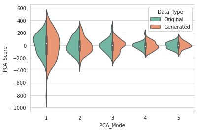
We will use a violin plot to visualize the difference in the real and augmented distributions.
DataAugmentationUtils.visualizeAugmentation(aug_data_csv, 'violin')
Example output:

Run data augmentation using a Mixture of Gaussian Distribution
output_directory = '../Output/MixtureAugmentation/'
sampler_type = "mixture"
embedded_dim = DataAugmentationUtils.runDataAugmentation(output_directory, img_list, world_particle_list, num_samples, num_dim, percent_variability, sampler_type)
aug_data_csv = output_directory + "/TotalData.csv"
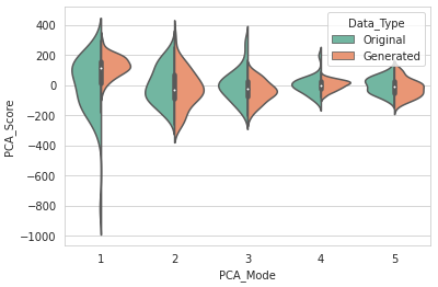
Visualize distribution of real and augmented data
DataAugmentationUtils.visualizeAugmentation(aug_data_csv, 'violin')
Example output:

Run data augmentation using Kernel Density Estimation
output_directory = '../Output/KDEAugmentation/'
sampler_type = "kde"
embedded_dim = DataAugmentationUtils.runDataAugmentation(output_directory, img_list, local_particle_list, num_samples, num_dim, percent_variability, sampler_type)
aug_data_csv = output_directory + "/TotalData.csv"
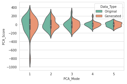
Visualize distribution of real and augmented data
DataAugmentationUtils.visualizeAugmentation(aug_data_csv, 'violin')
Example output:
