Getting Started with Exploring Segmentations¶

Before you start!¶

• This notebook assumes that shapeworks conda environment has been activated using conda activate shapeworks on the terminal.
• See Getting Started with Notebooks for information on setting up your environment and notebook shortcuts.
• See Getting Started with Segmentations to learn how to load and visualize binary segmentations.
• Note example output was generated on Linux/Mac environment and may look different on Windows.

In this notebook, you will learn:¶

1. How to define your dataset location and explore what is available in it
2. How to explore your dataset
3. How to decide the grooming pipeline needed for your dataset

In [ ]:

import shapeworks as sw

import shapeworks as sw

1. Defining and exploring your dataset¶

Defining dataset location¶

You can download exemplar datasets from ShapeWorks data portal after you login. For new users, you can register an account for free. Please do not use an important password.

After you login, click Collections on the left panel and then use-case-data-v2. Select the dataset you would like to download by clicking on the checkbox on the left of the dataset name. See the video below. After you download the dataset zip file, make sure you unzip/extract the contents in the appropriate location.

This notebook assumes that you have downloaded ellipsoid_1mode and you have placed the unzipped folder ellipsoid_1mode in Examples/Python/Data. Feel free to use your own dataset.

In [ ]:

#import relevant libraries
import os
import pyvista as pv
import numpy as np

# dataset name is the folder name for your dataset
datasetName  = 'ellipsoid_1mode'

# path to the dataset where we can find shape data 
# here we assume shape data are given as binary segmentations
shapeDir      = '../../Data/' + datasetName + '/segmentations/'
    
print('Dataset Name:     ' + datasetName)
print('Shape Directory:  ' + shapeDir)

#import relevant libraries import os import pyvista as pv import numpy as np # dataset name is the folder name for your dataset datasetName = 'ellipsoid_1mode' # path to the dataset where we can find shape data # here we assume shape data are given as binary segmentations shapeDir = '../../Data/' + datasetName + '/segmentations/' print('Dataset Name: ' + datasetName) print('Shape Directory: ' + shapeDir)

What is available in the dataset?¶

First let's see how many shapes we have in the dataset.

File formats: For binary segmentations, all itk-supported image formats can be used.

In [ ]:

import glob 
from pathlib import Path 


shapeExtention = '.nrrd'

# let's get a list of files for available segmentations in this dataset
# * here is a wild character used to retrieve all filenames 
# in the shape directory with the file extensnion
shapeFilenames = sorted(glob.glob(shapeDir + '*' + shapeExtention)) 

print ('Number of shapes: ' + str(len(shapeFilenames)))
print('Shape files found:')
for shapeFilename in shapeFilenames:
    shapeFilename = Path(shapeFilename)
    print(shapeFilename)

import glob from pathlib import Path shapeExtention = '.nrrd' # let's get a list of files for available segmentations in this dataset # * here is a wild character used to retrieve all filenames # in the shape directory with the file extensnion shapeFilenames = sorted(glob.glob(shapeDir + '*' + shapeExtention)) print ('Number of shapes: ' + str(len(shapeFilenames))) print('Shape files found:') for shapeFilename in shapeFilenames: shapeFilename = Path(shapeFilename) print(shapeFilename)

2. Exploring your dataset¶

We would like to better understand the given dataset to decide the appropriate grooming (preprocessing) pipeline/step to prepare it for shape modeling.

Loading your dataset¶

First step is to load the dataset.

Note: If your dataset is large (large volumes and/or large number of segmentations), you could select a subset for this exploration step.

In [ ]:

# list of shape segmentations
shapeSegList = []

# list of shape names (shape files prefixes) to be used 
# for saving outputs and visualizations
shapeNames   = [] 

# loop over all shape files and load individual segmentations
for shapeFilename in shapeFilenames:
    print('Loading: ' + shapeFilename)
    
    # current shape name
    segFilename = shapeFilename.split('/')[-1] 
    shapeName   = segFilename[:-len(shapeExtention)]
    shapeNames.append(shapeName)
    
    # load segmentation
    shapeSeg = sw.Image(shapeFilename)
    
    # append to the shape list
    shapeSegList.append(shapeSeg)

num_samples = len(shapeSegList)
print('\n' + str(num_samples) + 
      ' segmentations are loaded for the ' + datasetName + ' dataset ...')

# list of shape segmentations shapeSegList = [] # list of shape names (shape files prefixes) to be used # for saving outputs and visualizations shapeNames = [] # loop over all shape files and load individual segmentations for shapeFilename in shapeFilenames: print('Loading: ' + shapeFilename) # current shape name segFilename = shapeFilename.split('/')[-1] shapeName = segFilename[:-len(shapeExtention)] shapeNames.append(shapeName) # load segmentation shapeSeg = sw.Image(shapeFilename) # append to the shape list shapeSegList.append(shapeSeg) num_samples = len(shapeSegList) print('\n' + str(num_samples) + ' segmentations are loaded for the ' + datasetName + ' dataset ...')

Visualizing your dataset¶

Now let's visualize all samples in a grid using pyvista. You may need to call pv.close_all() every once in a while to clean up the unclosed plotters. We will use sw.plot_volumes function from the Shapeworks python module. This function will take in a list of shapeworks images as input and initiate a pyvista plotter to render multiple windows, each with a single segmentation, add segmentations to the plotter, and start rendering.

In [ ]:

# define parameters that controls the plotter
use_same_window = False # plot using multiple rendering windows if false
notebook        = False # True will enable the plots to lie inline
show_borders    = True  # show borders for each rendering window
shade_volumes   = True  # use shading when performing volume rendering
color_map       = "viridis" # color map for volume rendering, e.g., 'bone', 'coolwarm', 'cool', 'viridis', 'magma'
show_axes       = True  # show a vtk axes widget for each rendering window
show_bounds     = True  # show volume bounding box
show_all_edges  = True  # add an unlabeled and unticked box at the boundaries of plot. 
font_size       = 10    # text font size for windows
link_views      = True  # link all rendering windows so that they share same camera and axes boundaries

# plot all segmentations in the shape list
sw.plot_volumes(shapeSegList,    
             volumeNames     = shapeNames, 
             use_same_window = use_same_window,
             notebook        = notebook,
             show_borders    = show_borders,  
             shade_volumes   = shade_volumes, 
             color_map       = color_map,
             show_axes       = show_axes,  
             show_bounds     = show_bounds,
             show_all_edges  = show_all_edges, 
             font_size       = font_size,   
             link_views      = link_views
             )

# define parameters that controls the plotter use_same_window = False # plot using multiple rendering windows if false notebook = False # True will enable the plots to lie inline show_borders = True # show borders for each rendering window shade_volumes = True # use shading when performing volume rendering color_map = "viridis" # color map for volume rendering, e.g., 'bone', 'coolwarm', 'cool', 'viridis', 'magma' show_axes = True # show a vtk axes widget for each rendering window show_bounds = True # show volume bounding box show_all_edges = True # add an unlabeled and unticked box at the boundaries of plot. font_size = 10 # text font size for windows link_views = True # link all rendering windows so that they share same camera and axes boundaries # plot all segmentations in the shape list sw.plot_volumes(shapeSegList, volumeNames = shapeNames, use_same_window = use_same_window, notebook = notebook, show_borders = show_borders, shade_volumes = shade_volumes, color_map = color_map, show_axes = show_axes, show_bounds = show_bounds, show_all_edges = show_all_edges, font_size = font_size, link_views = link_views )

3. Deciding the grooming pipeline needed for your dataset¶

Does this dataset need grooming? What are grooming steps needed? Let's inspect the segmentations. What do we observe?

Voxel spacing¶

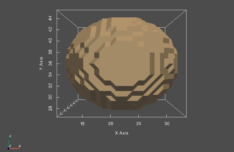
Voxel spacing are not isotropic, i.e., voxel size in each of the three dimensions are not equal.This can be identified if you zoom-in in the visualization below and observe the step size in the x,y,z direction. Anisotropic spacing could adversely impact particles optimization since shapeworks assumes equal voxel spacing. Some datasets might also have different voxel spacings for each segmentation.

Hence, it is necessary to bring all segmentations to the same voxel spacing that is equal in all dimensions.

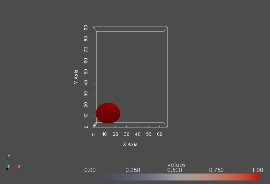
Another observation is voxel spacing is relatively large. This can be observed by the pixelated volume rendering and the jagged isosurface.

We can improve the segmentation resolution by decreasing voxel spacing.

In [ ]:

import pyvista as pv
# to better appreciate the pixelated nature of these segmentations, we need to only visualize 
# the binary segmentation, notice the thick slices

shapeIdx = 10
shapeSeg = shapeSegList[shapeIdx]
 

shapeSeg_vtk = sw.sw2vtkImage(shapeSeg, verbose = True)

sw.plot_volumes(shapeSeg_vtk)

import pyvista as pv # to better appreciate the pixelated nature of these segmentations, we need to only visualize # the binary segmentation, notice the thick slices shapeIdx = 10 shapeSeg = shapeSegList[shapeIdx] shapeSeg_vtk = sw.sw2vtkImage(shapeSeg, verbose = True) sw.plot_volumes(shapeSeg_vtk)

Segmentations and image boundaries¶

Some segmentations are very close to the image boundary, not leaving enough room for particles (correspondences) to move and spread over these surface regions. In particular, particles could overshoot outside the image boundary during optimization.

Furthermore, if a segmentation touches the image boundary, this will result in an artificially (i.e., not real) open surface.

Hence, these segmentations needs to be padded with background voxels (zero-valued) to create more room along each dimension.

In [ ]:

# let's inspect a segmentation that touches the image boundaries
shapeIdx = 13
shapeSeg = shapeSegList[shapeIdx]

shapeSeg_vtk = sw.sw2vtkImage(shapeSeg, verbose = False)

sw.plot_volumes(shapeSeg_vtk)

# let's inspect a segmentation that touches the image boundaries shapeIdx = 13 shapeSeg = shapeSegList[shapeIdx] shapeSeg_vtk = sw.sw2vtkImage(shapeSeg, verbose = False) sw.plot_volumes(shapeSeg_vtk)

This segmentation touches the image boundary and hence will result in an artificially open surface. To inspect this behavior, we need extract a surface mesh (isosurface) from each segmentation. An isosurface is a three-dimensional surface that represents points of a constant value (aka isovalue) within the given volume of space.

In [ ]:

# let's see if there's a function that extracts an isosurface from an image
# use dot-tap to get a list of functions/apis available for shapeSeg

# found it - toMesh, let's see its help
help(shapeSeg.toMesh)

# let's see if there's a function that extracts an isosurface from an image # use dot-tap to get a list of functions/apis available for shapeSeg # found it - toMesh, let's see its help help(shapeSeg.toMesh)

The toMesh function needs an isovalue, which is the constant value the represents the surface of interest. Since a shape segmentation is a binary image, the foreground is expected to have the value of 1 (white) and the background should have a zero value (black), so an appropriate isovalue to extract the foregound-background interface a value in between, e.g., 0.5

In [ ]:

import numpy as np
# let's make sure that our assumptions about the voxel values are correct
# is the given volume a binary segmentation?

# first convert to numpy array
shapeSeg_array = shapeSeg.toArray()

# make sure that it is a binary segmentation
voxelValues = np.unique(shapeSeg_array)
print('\nVoxel values:' + str(voxelValues))

if len(voxelValues) > 2:
    print('WARNING: ' + shapeName + ' is not a bindary segmentation. Voxels have more than two distinct values')
    print('PLEASE make sure to use binary segmentations')
else:
    print('Shape ' + shapeName + ' is a binary segmentation')

import numpy as np # let's make sure that our assumptions about the voxel values are correct # is the given volume a binary segmentation? # first convert to numpy array shapeSeg_array = shapeSeg.toArray() # make sure that it is a binary segmentation voxelValues = np.unique(shapeSeg_array) print('\nVoxel values:' + str(voxelValues)) if len(voxelValues) > 2: print('WARNING: ' + shapeName + ' is not a bindary segmentation. Voxels have more than two distinct values') print('PLEASE make sure to use binary segmentations') else: print('Shape ' + shapeName + ' is a binary segmentation')

In [ ]:

# now define the isovalue, in case a binary segmentation has a foreground label that is not 1
# we need to obtain a value inbetween

# get min and max values
minVal = shapeSeg_array.min()
maxVal = shapeSeg_array.max()

print('\nMinimum voxel value: ' + str(minVal))
print('Maximum voxel value: ' + str(maxVal))

isoValue = (maxVal - minVal)/2.0
print('\nisoValue = ' + str(isoValue))

# now define the isovalue, in case a binary segmentation has a foreground label that is not 1 # we need to obtain a value inbetween # get min and max values minVal = shapeSeg_array.min() maxVal = shapeSeg_array.max() print('\nMinimum voxel value: ' + str(minVal)) print('Maximum voxel value: ' + str(maxVal)) isoValue = (maxVal - minVal)/2.0 print('\nisoValue = ' + str(isoValue))

In [ ]:

# let's extract the segmentation isosurface and visualize it

# extract isosurface
shapeMesh = shapeSeg.toMesh(isovalue = isoValue)
 
# sw to vtk
shapeMesh_vtk = sw.sw2vtkMesh(shapeMesh)

sw.plot_meshes([shapeMesh_vtk])

# let's extract the segmentation isosurface and visualize it # extract isosurface shapeMesh = shapeSeg.toMesh(isovalue = isoValue) # sw to vtk shapeMesh_vtk = sw.sw2vtkMesh(shapeMesh) sw.plot_meshes([shapeMesh_vtk])

So, we have been able to extract a segmentation's isosurface and visualize it as a surface mesh. It is worth noting that the jagged surface is due to the anisotropic voxel space (with spacing in z-dimension is double that of x- and y-dimensions) and large voxel size.

Shape alignment¶

One can observe from the segmentation visualization that they are not roughly aligned, i.e., they do not share the same coordinate frame where each individual shape is located differently compared to other shapes.

Aligning shapes is a critical preprocessing step to avoid the shape model to encode variabilities pertaining to global transformations such as rotation and translation.

In [ ]:

# let's inspect some segmentations where we can observe misalignment
shapeIdxs = [8,9,10]

shapeSegSubset   = [shapeSegList[shapeIdx] for shapeIdx in shapeIdxs ]
shapeNamesSubset = [shapeNames[shapeIdx]   for shapeIdx in shapeIdxs ]

# let's inspect some segmentations where we can observe misalignment shapeIdxs = [8,9,10] shapeSegSubset = [shapeSegList[shapeIdx] for shapeIdx in shapeIdxs ] shapeNamesSubset = [shapeNames[shapeIdx] for shapeIdx in shapeIdxs ]

To inspect how mutliple segmentation are spatially aligned with respect to each other, we will visualize their surfaces in the same rendering window.

In [ ]:

shapeSegIsosurfaces     = []
shapeSegIsosurfaces_vtk = []

for shapeSeg in shapeSegSubset:
    
    # extract isosurface
    shapeIsosurface = shapeSeg.toMesh(isovalue = isoValue)
    
    shapeSegIsosurfaces.append(shapeIsosurface)
 
    # sw to vtk
    shapeSegIsosurfaces_vtk.append(sw.sw2vtkMesh(shapeIsosurface, verbose = False))

shapeSegIsosurfaces = [] shapeSegIsosurfaces_vtk = [] for shapeSeg in shapeSegSubset: # extract isosurface shapeIsosurface = shapeSeg.toMesh(isovalue = isoValue) shapeSegIsosurfaces.append(shapeIsosurface) # sw to vtk shapeSegIsosurfaces_vtk.append(sw.sw2vtkMesh(shapeIsosurface, verbose = False))

In [ ]:

sw.plot_meshes(shapeSegIsosurfaces,       
            use_same_window = True, 
            notebook        = False,  
            show_borders    = True,  
            meshes_color    = ['tan', 'blue','red'], 
            mesh_style      = "surface", 
            show_mesh_edges = False, 
            show_axes       = True,  
            show_bounds     = True,  
            show_all_edges  = True,  
            font_size       = 10,    
            link_views      = True   
           )

sw.plot_meshes(shapeSegIsosurfaces, use_same_window = True, notebook = False, show_borders = True, meshes_color = ['tan', 'blue','red'], mesh_style = "surface", show_mesh_edges = False, show_axes = True, show_bounds = True, show_all_edges = True, font_size = 10, link_views = True )

Too much background¶

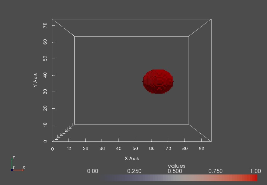
Image boundaries are not tight around shapes, leaving irrelevant background voxels that might increase the memory footprint when optimizing the shape model.

We can crop segmentations to remove unnecessary background.

In [ ]:

shapeIdx = 12
shapeSeg = shapeSegList[shapeIdx]

shapeSeg_vtk = sw.sw2vtkImage(shapeSeg, verbose = False)

sw.plot_volumes(shapeSeg_vtk)

shapeIdx = 12 shapeSeg = shapeSegList[shapeIdx] shapeSeg_vtk = sw.sw2vtkImage(shapeSeg, verbose = False) sw.plot_volumes(shapeSeg_vtk)

Binary segmentations¶

In general, this binary representation is not useful for finite numerical calculation of surface geometry and features that are required in shape modeling, which assumes the image is a sampling of a smooth function.

Hence, ShapeWorks makes use of the signed distance transform of the binary segmentation that does satisfy this criterion.

For the correspondence optimization step, shapes can be represented as the zero level set of a smooth signed distance transform.

Tentative grooming¶

Hence, a tentative grooming pipeline entails the following steps:

1. Resampling segmentations to have smaller and isotropic voxel spacing
2. Rigidly aligning shapes
3. Cropping and padding segmentations
4. Converting segmentations to smooth signed distance transforms

Let the fun begins!!! Please visit Getting Started with Grooming Segmentations to learn how to groom your dataset.